Visualizing HoG Features

Finished writing some of the code for HoG features. Still haven't completely understood/implemented the portion for detection via sliding window.

The following outlines our process: (more information at http://en.wikipedia.org/wiki/Histogram_of_oriented_gradients)

Gradient maps are first computed using Sobel operator or 1-D derivative masks.

gradient in x-direction

gradient in y-direction

Using these gradient maps, we can calculate a magnitude and orientation for every pixel. We bin these pixels based on the angle of orientation, using nine bins (increments of 20 degrees, 0 to 180).

Then we group pixels together into "cells" and the orientation of the cell is determined by the magnitudes of the pixels within that cell. Here are some visual representations of HoG features of an image.
The bin with the highest magnitude for each cell is chosen to represent that cell:

Original image

16x16 pixel cells

8x8 pixel cells

4x4 pixel cells

Here are some more examples (original on left, HoG on right)

 

In recent years, a lot of people have reached out to me for guidance on how to generate these HOG visualizations. Please take a look at https://github.com/Porkbutts/Vespidae-Wasp-Classification/blob/master/Project/practice.cpp#L223 if you are interested.

Working with manually pre-processed images

I got the photoshopped wasps without wings/legs/antennae. Some of them are not so clean, so I have excluded those, but most of them are very good.

After experimented with classification on these images, here are some of the results. Using only color histograms, classification improved to about 80%. This is probably due to the color of wings varying from specimen to specimen, the classifier no longer has to deal with this issue.

Using simple HoG features, classification is about 55% accurate. Here is the confusion matrix using a nearest neighbor classifier on only HoG features:

Note that, even though classification results are not very high, they make sense.

Many examples from class 3 are misclassified as class 8 due to their similar body type:

Also class 4 misclassified as class 5:

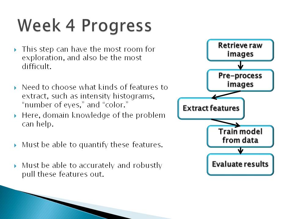
Using Histogram of Oriented gradients, the image is divided into many overlapping blocks. This type of approach could also be applied to the color histograms. From here we can scan the image for body parts such as abdomen/head/etc... if we have a database of trained parts.

Restructuring the project

Sorry I haven't had much time to update the blog.

I am attaching some of the slides from my weekly progress report as a series of images as most of what I have to say would be redundant. I discuss the workflow necessary for a fully automated image classification system, and the step in that pipeline that I will be focusing on.

At the start of the week, I tried to look into identifying different parts of the insect, such as head/thorax/abdomen. Professor David Kriegman (UCSD Computer Vision) pointed me into the direction of a part-modeling paper: http://www.cs.cornell.edu/~dph/papers/pict-struct-ijcv.pdf
Professor Serge Belongie (UCSD Computer Vision) suggested I take a look at HoG features (Histogram of Oriented gradients: http://en.wikipedia.org/wiki/Histogram_of_oriented_gradients#Gradient_computation)

I also looked into this paper on part-modeling using HoG features:
http://ttic.uchicago.edu/~dmcallester/lsvm-pami.pdf

I've been trying to write code for extracting HoG features, since OpenCV only provides code for extracting descriptors. I would like to manipulate the features manually and play around with them, so that is why I am writing code for it. I hope to have the code for HoG features implemented by next week and some images of the histograms that I can show for demonstration.

Exploring SIFT

SIFT stands for Scale Invariant Feature Transform. It is a patented algorithm that looks for feature points or "interest" points  in an image. These points of interest are independent of image scale, rotation, and illumination and are also quick to compute, making them very robust features.

Each feature point has a scale and orientation. From these images, scale is denoted by the size of the circle, and orientation is denoted by the direction of its radius. Here are some examples of SIFT features detected using OpenCV.

From the images, there are too many cluttered feature points, so it might be best to choose the most important ones, and leave out others. Next time I will try to use these SIFT features to detect bilateral symmetry, and other key features.

Extracting Patterns based on Colors

Recently I have been looking into thresholding based on colors.

Running histogram equalization on each channel of an image produces the following images (upper left, bottom left, bottom middle). Combining these images back into one color image produces the "equalized" image (top-middle). As one will notice, the colors that represent the patterns stand out brightly, and from here we can simply threshold the image into a binary image (upper-right).

Taking this idea further, we can choose a region of interest near the centroid of the image, to look for patterns on the back of the insect. This is noted by the red square on bottom-most image. The patterns in the binary image are taken from this square and edge-detection is performed, resulting in the small square (upper-right).

No noticeable patterns near center

Back pattern slightly detected.

Back pattern noticeable and extracted.

Tweaking Performance: Auto-contrast and Regions of Interest

To tweak the performance of the classifier, I have added two pre-processing steps to the feature extraction.

The first is auto-contrast, which is a means of "stretching" the histogram so that the last filled bin is now at location 255. We do this on each channel, here are some images before and after auto-contrast:

 

 

 

 

 

 

This process of auto-contrast helps to produce a better binary image for masking purposes.

Since the wings were producing inconsistent colors, the second pre-processing step I have added is to use a region of interest to extract the histograms. For this I chose a rectangular box located approximately around the center of the wasp. Histograms are extracted from this region, so not only is it more descriptive of the wasp class, but it is also more efficient to calculate (less pixels to iterate over).

Here are some images showing the ROI (Region of Interest). Also note that background pixels are not included in the histogram calculation as the binary image masks them out.

 

 

Results Analysis:

At first I considered making the rectangle a square so wasp orientation would not affect the feature space. When I did that the performance increased only about 2%, but since then I have removed the vertically oriented wasps to simplify the problem for now. The performance increased by about 5% on the nearest neighbor classifier after making these adjustments (may be due to the changing of the image set).